Geological timescale axis guide — guide

guide_geo behaves similarly to ggplot2::guide_axis() in that it modifies the visual appearance of the axis. The main difference is that it adds a geological timescale instead of an axis.

Usage

guide_geo(
  dat = "periods",
  fill = NULL,
  alpha = 1,
  height = unit(2, "line"),
  bord = c("left", "right", "top", "bottom"),
  lwd = 0.25,
  color = "black",
  lab = TRUE,
  lab_color = NULL,
  rot = 0,
  family = "sans",
  fontface = "plain",
  size = 5,
  skip = c("Quaternary", "Holocene", "Late Pleistocene"),
  abbrv = TRUE,
  neg = FALSE,
  end_labels = "center",
  dat_is_discrete = FALSE,
  fittext_args = list(),
  theme = NULL,
  title = waiver(),
  order = 0,
  position = waiver()
)

Arguments

dat: Either A) a string indicating a built-in dataframe with interval data from the ICS ("periods", "epochs", "stages", "eons", or "eras"), B) a string indicating a timescale from macrostrat (see list here: https://macrostrat.org/api/defs/timescales?all), or C) a custom data.frame of time interval boundaries (see Details).
fill: The fill color of the boxes. The default is to use the color column included in dat. If a custom dataset is provided with dat without a color column and without fill, a greyscale will be used. Custom fill colors can be provided with this option (overriding the color column) and will be recycled if/as necessary.
alpha: The transparency of the fill colors.
height: The height (or width if pos is left or right) of the scale.
bord: A vector specifying on which sides of the scale to add borders (same options as pos).
lwd: Line width.
color: The outline color of the interval boxes.
lab: Whether to include labels.
lab_color: The color of the labels. The default is to use the lab_color column included in dat. If a custom dataset is provided with dat without a lab_color column and without fill, all labels will be black. Custom label colors can be provided with this option (overriding the lab_color column) and will be recycled if/as necessary.
rot: The amount of counter-clockwise rotation to add to the labels (in degrees).
family: The font family to use for the labels. There are only three fonts that are guaranteed to work everywhere: “sans” (the default), “serif”, or “mono”.
fontface: The font face to use for the labels. The standard options are "plain" (default), "bold", "italic", and "bold.italic".
size: Label size. Either a number as you would specify in ggplot2::geom_text() or "auto" to use ggfittext::geom_fit_text().
skip: A vector of interval names indicating which intervals should not be labeled. If abbrv is TRUE, this can also include interval abbreviations.
abbrv: If including labels, should the labels be abbreviated? If TRUE, the abbr column will be used for the labels. If FALSE, the name column will be used for the labels. If "auto", the abbreviate() function will be used to abbreviate the values in the name column. Note that the built-in data and data retrieved via get_scale_data() already have built-in abbreviations. However, using the "auto" option here will create new unique abbreviations based on only the intervals that are being plotted. In many cases, this may result in abbreviations that are shorter in length because there are fewer similar interval names to abbreviate.
neg: Set this to TRUE if your x-axis is using negative values.
end_labels: How should labels for intervals at the ends of the guide be treated? "center", the default, centers the labels within the visible part of the label. "clip" removes the labels if their midpoint is beyond the axis limits. "keep" plots the labels in the midpoint of the full interval.
dat_is_discrete: Are the ages in dat already converted for a discrete scale?
fittext_args: A list of named arguments to provide to ggfittext::geom_fit_text(). Only used if size is set to "auto".
theme: A theme object to style the guide individually or differently from the plot's theme settings. The theme argument in the guide overrides, and is combined with, the plot's theme.
title: A character string or expression indicating a title of guide. If NULL, the title is not shown. By default (waiver()), the name of the scale object or the name specified in labs() is used for the title.
order: A positive integer of length 1 that specifies the order of this guide among multiple guides. This controls in which order guides are merged if there are multiple guides for the same position. If 0 (default), the order is determined by a secret algorithm.
position: Where this guide should be drawn: one of top, bottom, left, or right.

Details

If a custom data.frame is provided (with dat), it should consist of at least 3 columns of data. See data(periods) for an example.

The name column lists the names of each time interval. These will be used as labels if no abbreviations are provided.
The max_age column lists the oldest boundary of each time interval.
The min_age column lists the youngest boundary of each time interval.
The abbr column is optional and lists abbreviations that may be used as labels.
The color column is also optional and lists a color for the background for each time interval.
The lab_color column is also optional and lists a color for the label for each time interval.

If the axis of the time scale is discrete, max_age and min_age will automatically be converted to the discrete scale. In this case, the categories of the discrete axis should match the values in the name column. If the ages within dat are already discretized, you can set dat_is_discrete to TRUE to prevent this automatic conversion. This can be useful for adding a time scale where categories and time intervals are not 1:1.

Since this guide only plots the timescale and not ticks or an axis line, a call to this function should almost always be combined with a call to ggplot2::guide_axis() within a call to ggplot2::guide_axis_stack() (see Examples). Note that in most cases this has the same end result as a single call to coord_geo(); however, there are some use cases in which this may be more useful or allow for more customization. For example, users may wish to combine this guide in unique ways with other guides. Further, since coord_geo() doesn't work with radial/fan phylogenies (and coord_geo_radial() is quite different visually), this guide can be used to achieve the look of coord_geo() on a radial/fan phylogeny.

Examples

library(ggplot2)
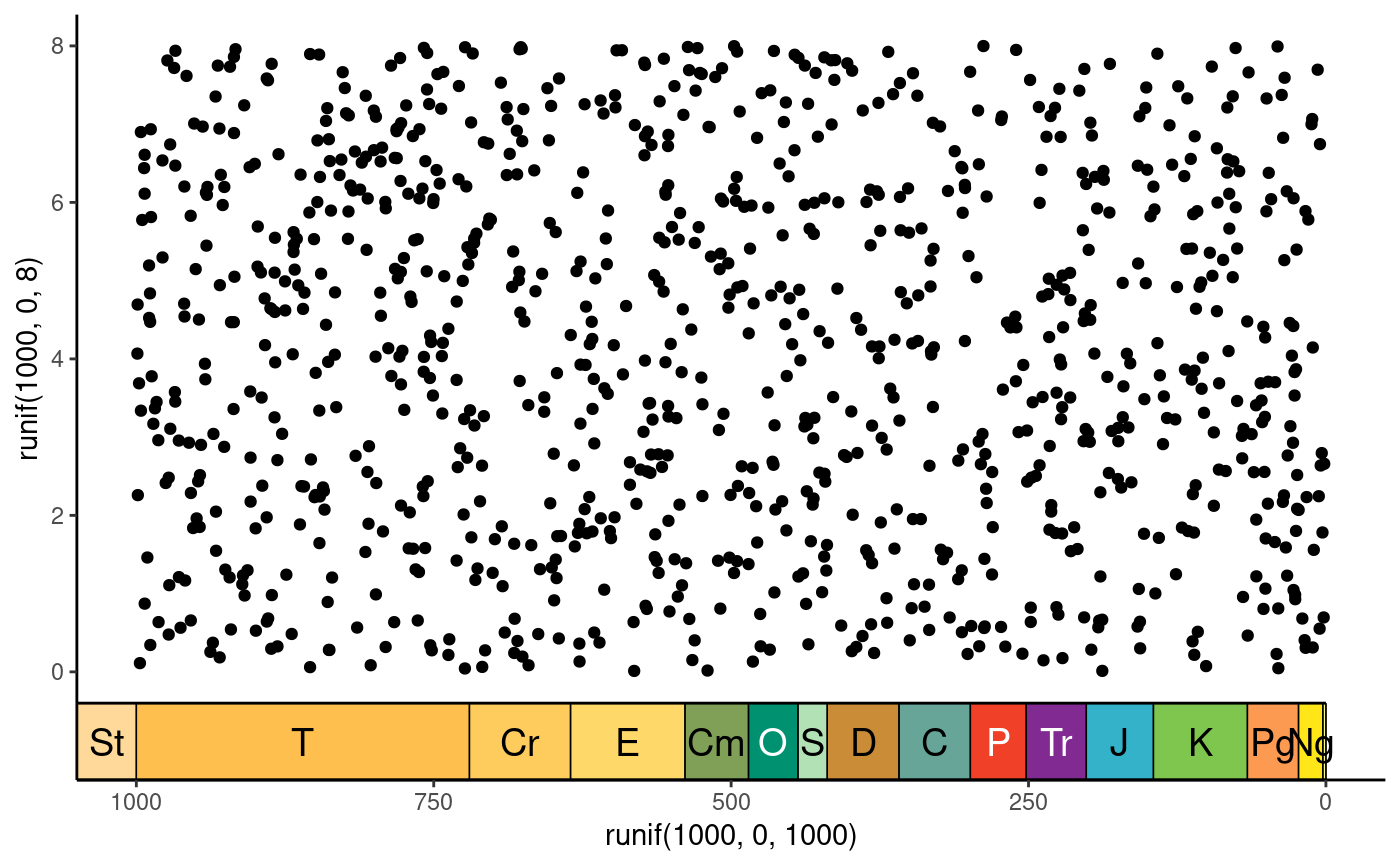
# reproduce the coord_geo() appearance
ggplot() +
  geom_point(aes(y = runif(1000, 0, 8), x = runif(1000, 0, 1000))) +
  scale_x_reverse(guide = guide_axis_stack(guide_geo(), "axis",
                  spacing = unit(0, "npc"))) +
  coord_cartesian(xlim = c(1000, 0), ylim = c(0, 8)) +
  theme_classic()

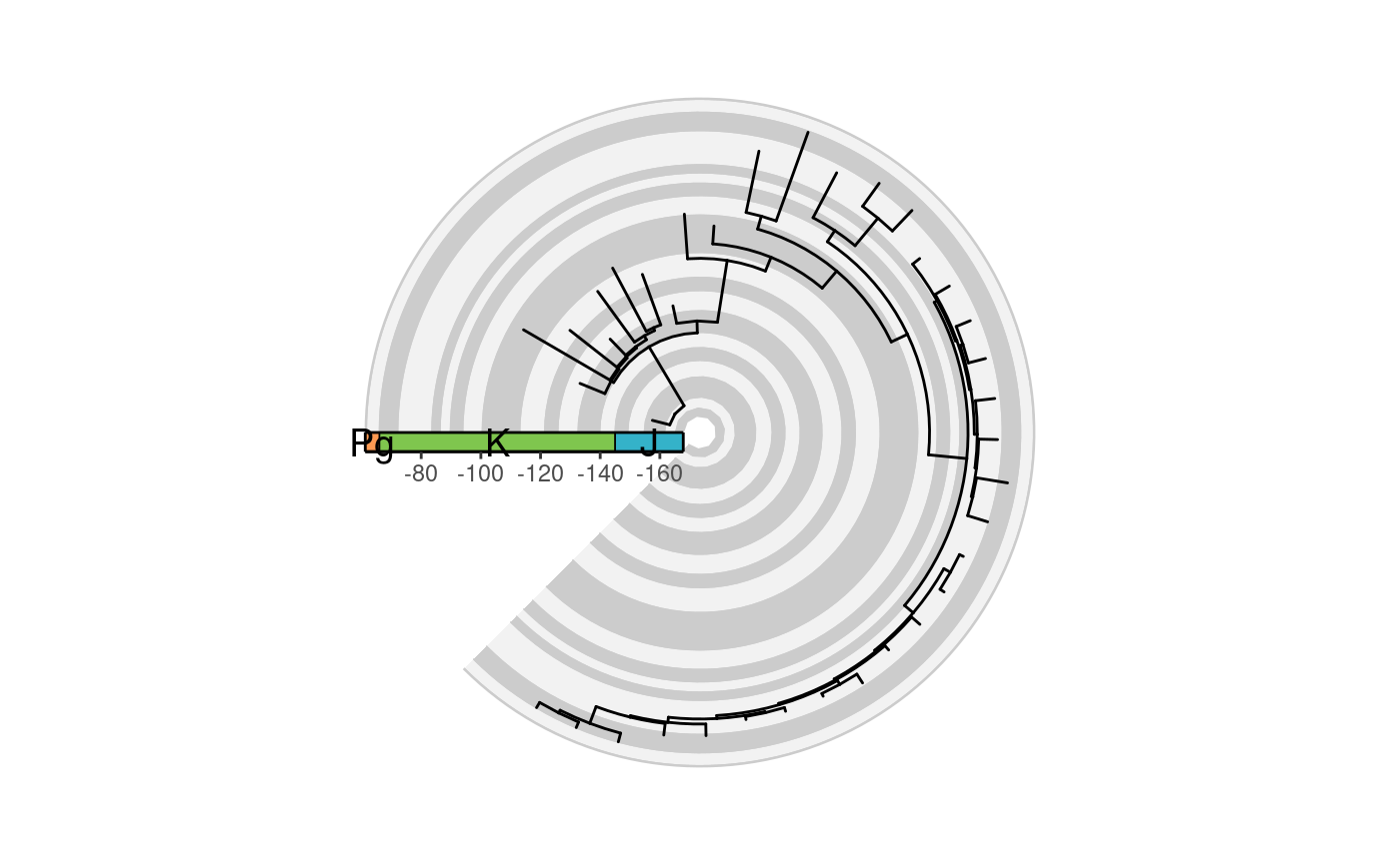
# the coord_geo() look on a radial phylogeny
library(ggtree)
library(paleotree)
data(RaiaCopesRule)
ggtree(ceratopsianTreeRaia,
       position = position_nudge(x = -ceratopsianTreeRaia$root.time)) +
  coord_geo_radial(dat = "stages", fill = c("grey80", "grey95"),
                   end = 1.25 * pi) +
  guides(
    r = guide_axis_stack(guide_geo(rot = -90, neg = TRUE,
                                   height = unit(0.5, "line")),
                         "axis", spacing = unit(0, "npc"))
  ) +
  scale_y_continuous(guide = "none", breaks = NULL) +
  theme_classic()
#> Scale for y is already present.
#> Adding another scale for y, which will replace the existing scale.